blobs

some axisymmetric simulations of a buoyant blob

Here are numerical (computer) simulations of a buoyant blob in a "can". The simulations are axisymmetric.

The purpose of the simulations is to demonstrate (to undergraduate meteorology students) the partitioning of buoyancy between driving vertical motion and sustaining a hydrostatic pressure deficit at the surface.

The can has a diameter equal to the height. The simulations are axisymmetric, meaning the variables in the (r,z) plane are forecasted. These variables are represented at 181 grid points in the vertical and 91 in the radial, uniformly distributed. The plotted fields are thus very smoothly varying.

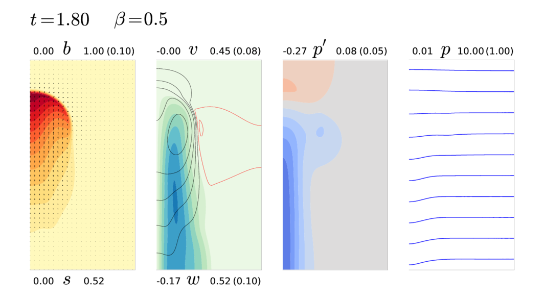
There are links to three animations below. Here is an example of what a frame looks like:

For those unfamiliar with axisymmetric simulations, what is shown here is the (r,z) plane. In a real "can", you would probably view the complete cross-section and see the blob at the center. Here we only need to show half of the cross-section, and the viewer should understand the mirror image also exists.

You may be unfamiliar with leaving units unspecified in simulations. One possible interpretation (among many) is to assume:

The diameter and height is 1 meter.
The buoyancy is provided by air that is about 10% higher temperature (at the center of the blob) than the ambient air, thus providing a potential vertical acceleration of 1 meter per second squared.
Time could be in units of seconds.
The air is assumed to have negligible viscosity, and the boundaries are assumed to be frictionless.

The symbols:

t, time
p pressure, minus the pressure in the upper right. The simulation is independent of the total pressure in the can. For example, the pressure could be 1000 atm or .001 atm.
p' pressure anomaly, pressure minus the ambient, undisturbed pressure far from the blob, at the same height
v the speed of the azimuthal wind
w the speed of the vertical wind
u the speed of the radial wind
s the speed of the wind in the (r,z) plane, √(u²+w²)

The labels:

For contour plots, the label shows the range of the variable and the contour increment.
For example 0.00 v 0.45 (.08) means v ranges between 0 and .45 and the contour interval is .08.
In all contour plots, a contour interval straddles zero, so in the above example for v, the first contour is at .04.
The color scheme for positive and negative values should be obvious.
v has filled contours, w has line contours.
p essentially displays the heights of isobaric surfaces, as familiar to meteorologists.
β is a parameter that controls the initialization of v

Explanation of β

The pressure in all simulations is initialized as hydrostatic, with the pressure constant at the top boundary. Thus puts a low pressure anomaly beneath the blob. A cyclostrophic v can be calculated that allows for a steady balance with the horizontal component of the pressure gradient force. β is a multiplier imposed on the calculated cyclostrophic v at the time of the initialization. Thus β=0 sets v=0, for which the hydrostatic initialization of pressure vanishes very quickly (after the first time step) because the speed of sound in the model is essentially infinite. The pressure in the model is calculated to keep the velocity field non-divergent. With β=1, the hydrostatic and cyclostrophic balance is perfectly compatible, and the initial fields can exist forever. With β=0.5 the initial cyclostrophic balance is weakened. This is the most interesting simulation.

animations of the simulations

There are many features to be seen in the simulations, that are probably best explained in a lecture.

β=1: initial perfect cyclostrophic balance Click "start", but nothing changes. A strong hurricane-like vortex perpetuates.
β=0: initial no cyclostrophic balance The buoyancy mainly goes into generating vertical wind. There is not much "severe" wind at the surface.
β=0.5: initial half cyclostrophic balance The vertical vorticity that is present at initialization is stretched into a strong vortex in the center of the domain. The vertical velocity in the core of the vortex is diminished. The buoyancy there is being used to maintain the low pressure in the vortex below.