Matched Asymptotic Expansion Compared with the Numerical Solution
The following equation is "too difficult" for Mathematica to find an analytical solution:
ε y'' + 2 y'  =0
=0
with y(0)=0 and y(1)=0.
When something is too difficult, Mathematica returns the command that was typed (after saying "running" in the top bar of the window for about 20 seconds).
So we solve the equation by a discrete numerical method, and by a method of matched asymptotic expansions. The ODE is a two-point boundary-value problem, which we solve using a shooting scheme.


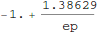
So we take out pencil and paper and find the following solution using matched asymptotic expansions:


Note the following property of our approximate solution. This information will be needed when we attempt to find a numerical solution.

To check our solution, we find a numerical solution for a particular value of ε. Mathematica solves ODE's by marching from initial conditions specified at a starting point. So we need to iterate to satisfy the condition y[1]=1/2 using what is called a "shooting method": we use  where we expect s will be a number near 1.


Let's try to use that InterpolatingFunction thing. The replacement rule for y is in a nested list. Let's evaluate it at t=0.3


As seen above, with s=1, our shooting scheme missed the boundary condition  . So we need to find the correct value of s.


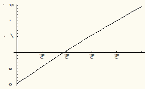


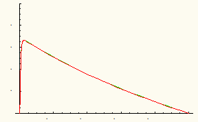
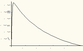
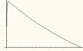
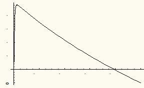
So we see that we have a numerical solution that satisfies both boundary conditions. Let's plot it out and compare it with our approximate solution.


Next we plot both the numerical and the perturbation solution together. They very nearly overlap: