Coupled oscillators,
jiggled from one end
A one-dimensional system of n masses connected by springs. The far end of the last spring, the spring connected to the right  , is fixed. The first spring, the spring connected to the left of
  , can be "jiggled" from the left with displacement
  . The system of equations to solve is :
 X = A X +F
where, for an example of 3 masses,

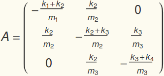
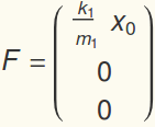
We can make this system dimensionless by using  as the time scale:
 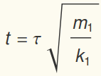 . The dimensionless system will be written as
 ,
,
where now all the  and
and  should be interpreted as the ratio of the dimensional value to
  and
and  , respectively. For example, if all
  and
and  , then

Also,

Let the eigenvectors of A be written as  and the eigenvalues be
  .
.
Construct a matrix P with the columns being the eigenvectors  .
.
Let X=P Y, which means Y is the amplitude of the eigenvectors that
are summed to represent the displacment. Here is the clever way
to solve the coupled problem:


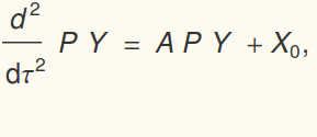
where D is a diagonal matrix of the eigenvalues. Let
 . This is really cool: there are uncoupled O.D.E.s for the amplitudes of each of the eigenvectors:

Finding a particular solution of the above equation is rather elementary.
We next present a technique for finding the homogeneous solution,
and in particular an efficient way to satisfy the initial conditions
 and
and  . The general homogeneous solution is:

where

Let  And let C be a column vector of the
  .
.


As a matrix problem, this gives

and

where Q=P D.
I like to turn off warnings about variable names being similar:
In[1]:=

In[2]:=

Create a matrix using "Input"-> "Create Table/Matrix/Pallette".
Then check "Matrix". The matrix is stored (and can also be input)
as a list of lists, with the inner lists being the rows of A. Comment
one of these A matrices as text, "uncomment" as needed. Note the
use of one decimal number forces the use of numerical computation, as opposed to
symbolic.
In[3]:=

Out[3]=


In[4]:=

Out[4]=

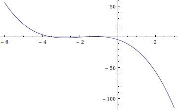
First, enjoy the exercise of finding eigenvalues without using the "canned" routine.
Note from the graph we expect negative roots for λ.
In[5]:=

Out[5]=

In[6]:=

Out[6]=

In[7]:=

Out[7]=

Or use the canned routine:
In[8]:=

Out[8]=

We will solve the homogeneous equation  by proposing
  . Obviously,
  . Let's make a list of these "eigenfrequencies":
In[9]:=

Out[9]=

Let Mathematica find the eigenvectors:
In[10]:=

Out[10]=

Store the eigenvectors are columns in P:
In[11]:=

Calculate  :
:
In[12]:=

Have a look at  :
:
In[13]:=

Out[13]//MatrixForm=

Have a look at  , just to see that it yields the expected diagonal matrix (except for round-off error):
In[14]:=

Out[14]//MatrixForm=

In[15]:=

Out[15]//MatrixForm=

In this particular example, we set  . In doing so, we have implicitly nondimensionalized displacement in terms of the amplitude of the "jiggle".
In[16]:=

Out[16]=

Project the forcing onto the eigenvectors:
In[17]:=

Out[17]=

A little "pencil and paper math" yields the amplitudes of the
eigenvectors as caused by the jiggling:
In[18]:=

Out[18]=

Let's consider a particular value of Ω, so that we can have something
to plot out:
In[19]:=

Out[19]=

In[20]:=

Out[20]=

In[21]:=

Out[21]=

In[22]:=

Out[22]=

In[23]:=

Out[23]=

In[24]:=

Out[24]=

Now with all the masses assumed to have no displacement and no velocity at t=0, we have
In[25]:=

Out[25]=

In[26]:=

Out[26]=

In[27]:=

Out[27]=

In[28]:=

Out[28]=

It is amazing what Mathematica can do with a list. Exp[list] makes a list. list*list makes a list of the product of the elements...
In[29]:=

Out[29]=

In[30]:=

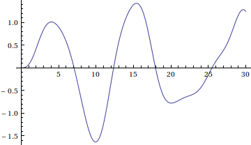
Check that we really did satisfy initial conditions:
In[31]:=

Out[31]=

In[32]:=

Out[32]=

In[33]:=

Out[33]=

In[34]:=

Out[34]=

In[35]:=

Out[35]=

In[36]:=

Out[36]=

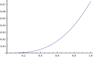
Check close up to see that initial conditions are really satisfied:
In[37]:=

Out[37]=

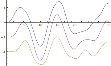
Here we plot all the X, with a shift added to the displacements to
make them easier to see. The shift makes a plot look like the
displacement from a common origin, as it might naturally appear
if the masses are hanging from a ceiling.
In[38]:=

In[39]:=

Out[39]=


 as the time scale:
  . The dimensionless system will be written as
 ,
,

